How To Create Sku In Excel

This post explores macro-free methods for using Excel's data validation feature to create an in-cell drop-down that displays choices depending on the value selected in a previous in-cell drop-down.

Overview

As with just about anything in Excel, there are several ways to achieve the goal. This post explores three such solutions, and if you have a preferred approach, please post a comment, I'd love to hear about it!

** NOTES:

• Beginning with Excel 2013 for Windows, we can use Slicers as an easier alternative to the solutions presented below. Please check out the Slicers post for more information.
• Another option is available in versions of Excel that include dynamic array functions and spill ranges. Please check out this post for more information.

The solutions we will explore are:

• One Table – hardest formulas; easiest ongoing data management; nonvolatile; removes blank choices
• Two Tables – easier formulas; harder ongoing data management; nonvolatile
• INDIRECT – easiest formulas; volatile; includes blank choices

The One Table approach stores all drop-down choices (for both the primary and secondary drop-downs) in a single table, but, the formulas are the hardest to set up initially. As a result, once the formulas are set up it is easy to add new primary and secondary drop-down choices without updating the formulas. This is the most "bulletproof" approach, and a good option to use when you have frequent changes to the drop-down choices or when you want to ensure that other users can easily add choices. Plus, you can remove blank choices from the drop-down.

The Two Tables approach stores the choices in two tables, and its formulas are a bit easier to set up initially. Special care must be taken when adding new drop-down choices, including adding new primary choices to two tables and ensuring the secondary table is sorted in ascending order. This is a good option when there are infrequent changes to the drop-down options or when you, the workbook administrator, will be updating the options and can be sure to resort the secondary table.

The INDIRECT approach uses the volatile INDIRECT function. The formulas in this approach are by far the easiest to implement initially, however, the INDIRECT function is volatile which means you may notice an overall performance decrease in your workbook depending on its size, the number of formulas, and so on. This option will include blank choices in the drop down. This is a good option when you want simple formulas and the workbook is relatively small. Note that with this approach, if you change the table name you would also need to update the related data validation formulas. Thanks Danny for your brilliant suggestion here!

We'll start with my preferred approach, the One Table approach. It is harder to set up initially, but once done, the choices are easier to manage over time. After we go through that approach, we'll discuss the Two Tables approach. It has easier formulas and is therefore easier to set up initially, but, the choices are more difficult to manage over time. We'll conclude with the INDIRECT option, which has the easiest formulas.

ONE TABLE Approach

The approach includes three Excel items working in harmony. The first task is storing the data validation choices in a table. The second is setting up named references that dynamically retrieve the correct data validation choices from the table. The third is setting up the data validation cells based on the defined names.

Alright, enough strategy, let's get into the tactics.

Storing Choices in a Table

First up is storing the drop-down choices in a table. The table feature was first introduced with Excel 2007, so, this approach only works with Excel versions 2007 and later.

The idea is that you store the choices for the first drop-down as table headers, and the choices for the second, dependent, drop-down as table data.

Let's get an illustration to provide something concrete. Let's use regions and reps. Our company has four regions, and within each region several reps. We are setting up a worksheet that allows a user to select a region, and then depending on the selected region, a rep. Thus, we need to set up a data validation drop-down that allows the user to select a valid region, and then a second drop-down that allows the user to select a valid rep.

We could store all of the data validation choices, both for the region drop-down and the rep drop-down in the following table, which is named tbl_choices for easy reference:

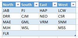
The benefits of storing the choices in a table like this are numerous. First and foremost, it is easy for users to modify the choices. Since tables auto-expand, any new choices added will be automatically included in the drop-downs, including new regions and reps. Column and row sort order doesn't matter, and the number of choices can vary in each column. One assumption is that there are no blank cells between reps.

Now that the choices are stored in a table, let's move on to creating the names that will be used by data validation.

Named References that Retrieve the Correct Choices

We have to set up some names that we can put into the data validation dialog box. Thus, these names need to return a valid range reference. Rather than set up unique names for each of the choices, we'll set up one name to use for the region drop-down, and one name for the rep drop-down. Once the names are set up, they won't need to be updated, and we don't need to add new names when a user adds new regions.

The first name is easy, since it simply refers to the headers row of the table. We can use the built-in structured table reference system to create this name.

We'll use the name manager (Formulas > Name Manager) to create a new name.

Our new name will be dd_regions and will reference the table's header row tbl_choices[#Headers], as illustrated in the screenshot below:

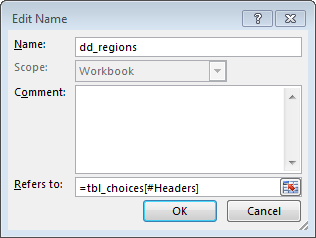
In just a moment, we'll use this custom name in the data validation for the region cell.

Now, let's create the name we need for the rep drop-down. In order to set up the name, we'll need to be familiar with these worksheet functions:

• INDEX
• MATCH

Let's see what we need the formula to accomplish, and then we'll see how these functions help.

Easy Version

We need a formula that will retrieve the column values for the selected region. This is pretty easy if we want to return all rows, even blank ones. We'll start with that. After we get that working, we'll enhance the formula to return only the rows with values, so that the drop-down list doesn't have a bunch of blank choices at the bottom.

The idea is that we need a formula that will return a column reference based on the table header. If you subscribe to this blog, this should sound familiar. We used a similar technique to dynamically feed a SUMIFS function based on the column header.

Essentially, we use the INDEX function to return a column reference, and we use the MATCH function to figure out which column. We'll store this formula as a named reference so that it is easy to use with data validation. Assuming that the selected region value is stored in cell C5, which we've named region for convenience, we'll add a new named reference dd_reps that references the following formula:

=INDEX(tbl_choices,,MATCH(region,dd_regions,0))

The INDEX function returns a range reference that starts with tbl_choices (argument #1), includes all rows (argument #2), and includes the column whose header matches the selected region (argument #3, computed by the MATCH function).

A screenshot is shown below for reference.

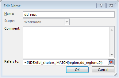
This named reference returns all of the cells in the selected region column, including any blank cells. This is the easy version, and before we move to the advanced version that excludes blank cells, let's set up the data validation.

Setting up Data Validation

Now that we have the two named formulas, we can simply set up data validation on the region and rep input cells.

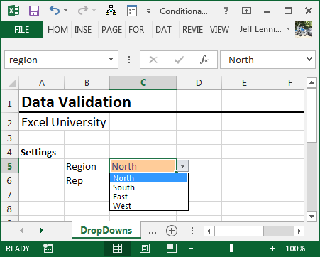
The data validation for the region input cell is set to allow a list equal to dd_regions, as displayed below:

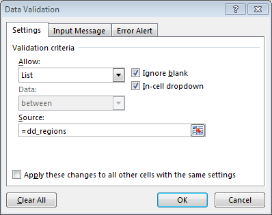
When we look at the worksheet, we see that it now provides a list of regions, as shown below:

So far so good! Now, for the big moment, the conditional rep drop-down, We set up data validation, and we allow a list equal to dd_reps, as shown below:

If the region cell is blank, you may receive an error alert message about the name evaluating to an error. You can safely click through the error dialog.

Now, when we return to the worksheet, we notice that the drop-down choices change depending on the selected region…wow…it worked! This is illustrated in the screenshot below:

And that my friend, is the basic version. It works well, except, I don't like how the drop-down includes blank cells. It would be better if we could somehow tell Excel to only include cells with values in the drop-down list. And we can, but it gets a little tricky. Let's explore this advanced version of the formula.

Advanced Version

If you'd like to exclude blank rows from the rep drop-down, we'll need to enhance our named formula.

Again, there are many approaches to this situation. One possible solution is to use the INDEX function to return a range, as follows.

It is easy to set up an A1-style range reference, you just specify the upper-left corner of the range and the lower-right corner of the range, such as A1:G12, or perhaps B5:D10. The INDEX function can similarly be used. We could use two INDEX functions to specify the range, for example: INDEX(…):INDEX(…). The first INDEX function returns a cell reference that represents the upper-left cell in the range, and the second INDEX function returns a cell reference that represents the lower-right cell in the range.

In order to make the formula we'll use with data validation easier to understand, we'll just write a couple of helper formulas and store them as names.

First, we'll need a shortcut for referencing the selected region column number. So, we set up a new name called dd_col_num that references the following formula:

=MATCH(region,dd_regions,0)

Now, anytime we need to know the column number of the selected region, we can simply refer to it with the name dd_col_num.

Next, we need a shortcut for referencing the selected region column. Not the column number, but, the entire table column. So, we set up a new name called dd_col that references the following formula:

=INDEX(tbl_choices,,dd_col_num)

Now, anytime we need to reference the selected region column, we can simply use dd_col.

Finally, we need a new name to use with the rep drop-down, and so we set up dd_reps2 to reference the following formula:

=INDEX(tbl_choices,1,dd_col_num) : INDEX(tbl_choices,COUNTA(dd_col),dd_col_num)

As you can see, we use the idea of INDEX(…):INDEX(…) to return the range. The first INDEX function returns the upper-left cell, and the second INDEX function returns the lower-right cell. The first INDEX function looks within tbl_choices (argument #1), and returns the cell reference at the intersection of the first table data row (argument #2) and the selected region column (argument #3, as calculated by the dd_col_num named formula).

The second INDEX function returns the cell within tbl_choices (argument #1), at the intersection of the last cell with data (argument #2, as computed by the COUNTA function) and the selected region column (argument #3).

With this in place, we can use data validation to allow a list equal to the name dd_reps2. This time, the drop-down excludes the blank cells, making us very happy.

This is illustrated in the screenshot below:

As an alternative to using the COUNTA function to count up the number of cells with values, we could use the MATCH function instead to find the last cell with data. To demonstrate this method, which would include any blank cells between reps, we set up a new name dd_reps3 as follows:

=INDEX(dd_col,1):INDEX(dd_col,MATCH("*",dd_col,-1))

As you can see, rather than try to get at the last rep with COUNTA, this approach uses MATCH instead, by matching a wildcard (*), in the rep column, and -1 for greater than. Check out the Excel help for the MATCH function for more details.

All three of these options, dd_reps, dd_reps2, and dd_reps3 are included in the download file below for reference.

TWO TABLES Approach

The two tables approach uses the same underlying Excel features and functions, including data validation, named ranges, and tables. However, the formulas are easier and thus this approach is easier to set up initially.

A summary of the steps are:

• Set up a table to store the primary drop-down choices named tbl_primary
• Set up a named range dd_primary that refers to tbl_primary
• Set up the primary drop-down input cell with data validation and allow a list equal to dd_primary
• Set up a table to store the secondary drop-down choices named tbl_secondary
• Set up a named range dd_secondary that retrieves the related choices
• Set up the secondary drop-down input cell with data validation and allow a list equal to dd_secondary

Here are the detailed steps.

First, we need to store the primary drop-down choices in a table named tbl_primary:

Next, we set up a new custom name dd_primary that refers to the table:

Then, we set up data validation on the primary input cell to allow a list equal to dd_primary:

The resulting primary input cell is shown below:

Now that the primary drop-down is working, let's tackle the secondary drop-down.

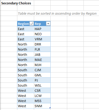
We set up the list of choices in a table named tbl_secondary, which must be sorted in ascending order by the primary column:

Next is the named range dd_secondary. This is the only tricky part. We'll use the INDEX/MATCH functions to figure out the related reps for the selected region. Since our primary input cell is stored in a worksheet named Two Tables in cell C6, we'll set up the name dd_secondary to refer to:

=INDEX(tbl_secondary[Rep],MATCH('Two Tables'!$C$6,tbl_secondary[Region],0),1): INDEX(tbl_secondary[Rep],MATCH('Two Tables'!$C$6,tbl_secondary[Region],1),1)

As you can see, this formula uses the range operator (:) to set up the range. The first cell in the range is determined by the first INDEX function. The last cell in the range is determined by the last INDEX function.

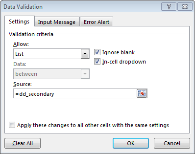
Then, we set up data validation on the secondary input cell to allow a list equal to dd_secondary:

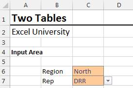
The resulting worksheet now contains conditional drop-down input cells:

Multiple Input Rows

As you can see, the above screenshot assumes only one entry, but, what if you needed to set this up so that users can enter multiple rows? No problem, the secret lies in the dd_secondary name.

While named ranges are often set up with absolute references, such as how the dd_secondary name used the absolute reference 'Two Tables'!$C$6, they can also be set up with relative references. When you set up a name with a relative reference, the active cell matters. That is, the active cell at the time you set up the name will indicate the base location for the relative reference. It is easy to visualize this idea by thinking about normal formulas. When you write a normal cell formula that uses a relative reference, the reference is relative to the cell that contains the formula. The same idea applies when setting up a named reference. The active cell, the one that is selected at the moment you open the new name dialog, will be used to determine how the relative cell reference is evaluated.

We can use this idea to set up multiple input rows. We create the dd_secondary name using a relative reference to the primary input cell while the active cell is the first secondary input cell:

Since our workbook already has a name dd_secondary, we'll use dd_secondary2 instead, and set the name equal to:

=INDEX(tbl_secondary[Rep],MATCH(Multiple!B7,tbl_secondary[Region],0),1): INDEX(tbl_secondary[Rep],MATCH(Multiple!B7,tbl_secondary[Region],1),1)

You'll notice in this version of the name, the MATCH function finds the value on the Multiple sheet in cell B7, which is a relative reference. Since the active cell when we set up the name was C7, the name will use the value to the left.

Now, when we set up data validation for the secondary input cells, we allow a list equal to dd_secondary2.

This is demonstrated in the sample file on the Multiple worksheet.

INDIRECT Approach

In this approach, we set up one table to store the primary drop-down choices in the header row and the related secondary choices in the columns. For illustration purposes, assume the table is named tbl_reps.

In the Data Validation list source box for the primary dropdown, you would use this:

=INDIRECT("tbl_reps[#Headers")

This tells data validation to convert the text string "tbl_reps[#Headers]" into the corresponding table reference to the header row. Please note that since the table name is embedded in the formula, if you change the table's name you would need to also update the data validation formula.

Assuming the primary drop down is stored in A1, you would then use the following formula in the secondary drop down's data validation list source

=INDIRECT("tbl_reps["&$A$1&"]")

The INDIRECT function here tells Excel to convert the text string into the structured table reference for the column name identified in A1.

The INDIRECT function is volatile, which means that it is updated each time the workbook is recalculated. This can be a performance hit in large workbooks. But, in small workbooks you shouldn't notice any performance hit and should work just fine.

Thanks Danny for this clean alternative solution!

This approach is demonstrated in the ConditionalDropDown3b workbook below.

Conclusion

The One Table and Two Tables approaches are two ways to provide dynamic drop-downs using Excel's data validation feature. If you have a preferred approach, or a way to simplify the formulas, please post a comment below!

Additional Resources

• To download the Excel file used for the screenshots above, which includes the table, named formulas, and data validation cells: ConditionalDropdown
• Multiple input rows example: ConditionalDropdown_2
  
• Using the INDIRECT approach: ConditionalDropdown3b
• Obtain the secondary drop-down list from a filtered PivotTable: ConditionalDropdownPT
• If you need to go more than two levels, you could simply continue this strategy and create drop-down choice tables for each additional dependent drop-down.
• If you haven't explored named references, tables, or data validation, these are all topics covered in the Excel University Volume 1 book and online Excel course.
• INDIRECT function to pull values from related tables

How To Create Sku In Excel

Source: https://www.excel-university.com/create-depdendent-drop-downs-conditional-data-validation/

Posted by: conefingir.blogspot.com

Share this post